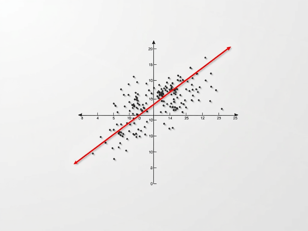
The image above was created using AI. More specifically, this was the first image generated by WordPress’ AI Image Generator, when given the prompt “Line of Best Fit Linear Regression”.

Linear regression is a foundational statistical technique used to model the relationship between two variables, allowing you to predict an unknown variable of a pair of variables given the the value of the other variable. I had already demonstrated how to do this with a specific dataset (Ice cream, in that case), but after following this simple tutorial, you should have a more general linear regression calculator that can predict pretty much any linear relationship!

Let’s break down the process step by step.

Understanding Linear Regression

Before diving into the code, let’s ensure we understand linear regression thoroughly. At its core, linear regression fits a straight line to a set of data points. The equation of this line is represented as:

y = mx + b

Where:

• y is the dependent variable,
• x is the independent variable,
• m is the slope of the line, and
• b is the y-intercept.

The goal of linear regression is to find the values of m and b that minimize the vertical distances between the observed data points and the line.

Collecting Data

The first step in our code is collecting data from the user. We prompt the user to input the number of data points they want to enter, and then gather pairs of x and y coordinates.

numdata = int(input("How many datapoints would you like to enter? "))
data_x = []
data_y = []
for i in range(numdata):
    data_x.append(int(input("Input x coordinate: ")))
    data_y.append(int(input("Input y coordinate: ")))

Here, we use a loop to iterate over the number of data points specified by the user. Inside the loop, we collect x and y coordinates and append them to separate lists.

Calculating the Line of Best Fit

Next, we calculate the slope (m) and y-intercept (b) of the line of best fit using the least squares method.

N = len(data_x)
sum_x = sum(data_x)
sum_y = sum(data_y)
sum_x_squared = sum([x ** 2 for x in data_x])
sum_xy = sum([x * y for x, y in zip(data_x, data_y)])

m = (N * sum_xy - sum_x * sum_y) / (N * sum_x_squared - sum_x ** 2)
b = (sum_y - m * sum_x) / N

Here, we compute the necessary sums (sum_x, sum_y, sum_x_squared, sum_xy) required for the least squares method. Then, we use these sums to calculate the slope (m) and y-intercept (b).

Visualizing the Data and Line of Best Fit

Finally, we visualize the original data along with the line of best fit using Matplotlib.

import matplotlib.pyplot as plt
import numpy as np

def make_plot(dx, dy, slope, intercept):
    x = np.linspace(min(dx), max(dx), 100)
    plt.scatter(dx, dy)
    plt.plot(x, slope * x + intercept, color='red')
    plt.xlabel(input("Input x axis name: "))
    plt.ylabel(input("Input y axis name: "))
    plt.title("Linear Regression")
    plt.grid(True)
    plt.show()

print("Plotting model (original data):")
make_plot(data_x, data_y, m, b)

Here, we define a function make_plot to create the plot. We generate a range of x values using np.linspace and plot the original data points as well as the line of best fit.

Conclusion

Building a simple linear regression calculator provides a hands-on understanding of how linear regression works. By breaking down the process into manageable steps, we’ve created a tool that can be used to analyze the relationship between two variables and make predictions based on observed data.