
The image above was created using AI. More specifically, this was the fourth image generated by Stable Diffusion, when given the prompt “Ice Cream Python Logistic Regression”.
Somewhat recently, I wrote some code for a Colab-assignment from my Applied AI in Python class, which I thought was pretty cool and was a good opportunity to understand the Linear Logistic Regression model.
So to start, we need something to model. This assignment in particular asked us to predict whether a soccer player would get injured based on the player’s age and the number of minutes the player plays.
Creating and Preparing the Data
Below is a very small dataset of 11 players, where each term in the list is a player, the first term of each sublist is the number of minutes played, the second term is player’s age, and the third term is whether or not a player was injured (with 1 meaning injured and 0 meaning not injured):
data = [
[78,32,0],
[34,27,1],
[78,21,1],
[79,28,1],
[75,21,0],
[43,24,1],
[13,29,1],
[17,37,0],
[70,32,0],
[85,23,0],
[63,30,0],
]
We can then convert this data from a python list to a pandas dataframe:
import pandas as pddf = pd.DataFrame(data, columns = ['average minutes', 'age', 'injured'])
Which allows us to assign column labels: average minutes, age, and injured. A plot of this data:

Now, we can prepare this dataset by converting the dataframe into an actually useable dataset using Numpy and Pandas.dataframe methods:
X = df.iloc[:, :-1]
y = df.iloc[:, -1]
X = np.c_[np.ones((X.shape[0], 1)), X]
y = y[:, np.newaxis]
theta = np.zeros((X.shape[1], 1))
Here, X represents the set of coordinates of each data point in the format [1., x_coordinate, y_coordinate], and y is a set of boolean indicators representing whether a point will be orange or blue in the format [0/1]. For now, theta is just a Numpy array with 0s. For completeness, we print these:
X: [[ 1. 78. 32.][ 1. 34. 27.][ 1. 78. 21.][ 1. 79. 28.][ 1. 75. 21.][ 1. 43. 24.][ 1. 13. 29.][ 1. 17. 37.][ 1. 70. 32.][ 1. 85. 23.][ 1. 63. 30.]]
y: [[0][1][1][1][0][1][1][0][0][0][0]]
theta: [[0.][0.][0.]]
Training the Model
To define the model, I used the Gradient Descent Logistic Regression class provided by my instructor:
import numpy as np
from scipy.optimize import fmin_tnc
class LogisticRegressionUsingGD:
    def sigmoid(x):
        return 1 / (1 + np.exp(-x))
    def net_input(theta, x):
        return np.dot(x, theta)
    def probability(self, theta, x):
        return self.sigmoid(self.net_input(theta, x))
    def cost_function(self, theta, x, y):
        m = x.shape[0]
        total_cost = -(1 / m) * np.sum(
            y * np.log(self.probability(theta, x)) + (1 - y) * np.log(1 - self.probability(theta, x)))
        return total_cost
    def gradient(self, theta, x, y):
        m = x.shape[0]
        return (1 / m) * np.dot(x.T, self.sigmoid(self.net_input(theta, x)) - y)
    def fit(self, x, y, theta):
        opt_weights = fmin_tnc(func=self.cost_function,  x0=theta, fprime=self.gradient, args=(x, y.flatten()))
        self.w_ = opt_weights[0]
        return self
    def predict(self, x):
        theta = self.w_[:, np.newaxis]
        return self.probability(theta, x)
    def accuracy(self, x, actual_classes, probab_threshold=0.5):
        predicted_classes = (self.predict(x) >= probab_threshold).astype(int)
        predicted_classes = predicted_classes.flatten()
        accuracy = np.mean(predicted_classes == actual_classes)
        return accuracy * 100
Finally, to derive the model’s three parameters, we use the following code:
model = LogisticRegressionUsingGD()
model.fit(X, y, theta)
accuracy = model.accuracy(X, y.flatten())
parameters = model.w_
Printing these, we get:The accuracy of the model is 81.81818181818183% The model parameters using Gradient descent: [12.29519714 -0.06191132 -0.3272452 ]
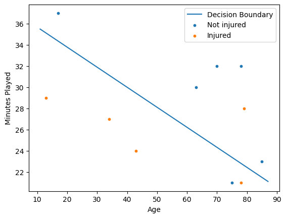
Plotting the model’s decision boundary, we get:
How cool!
