The image above was created using AI. More specifically, this was the fourth image generated by Stable Diffusion, when given the prompt “Neural Networks Harvard”.

It’s almost been two weeks since the end of my CSCI S-80 class, so I felt that this would be a good time to talk about one of the most interesting but puzzling units we covered in this class: neural networks.

Neural networks, which are also referred to as artificial neural networks or simulated neural networks, represent a specialized branch of machine learning (which is a specialized branch of AI), and serve as the core of deep learning algorithms. As one could tell from their name, the design of neural networks takes inspiration from the human brain- they replicate the intricate signaling between biological neurons.

This aspect of connection with the biological brain is quite apparent in the architecture and nomenclature of neural networks. These networks consist of layers of nodes, encompassing an input layer, one or more concealed layers, and an output layer. Each node, an artificial neuron, establishes connections with others, characterized by unique weights and thresholds. When a node’s output surpasses its designated threshold, it activates, transmitting data to the subsequent network layer. Conversely, outputs below the threshold withhold data transfer. Neural networks can be found in both Google’s famed search engine, and also in large language models like ChatGPT.

But how is a neural network actually structured?

Neural Network Structure

In their most basic form, neural networks, like functions, sum up inputs to produce an outputs.

In the above image, the two units on the left (represented by two white circles) are connected to an output unit on the right (represented by one white circle) in such a way that they are each weighted based on their corresponding weighted edges. The output, considering the values of both inputs multiplied by their weights, then uses the function g to choose an output.

Technically speaking, this is, by itself, a very simple neural network. Here is the same example with some values plugged in:

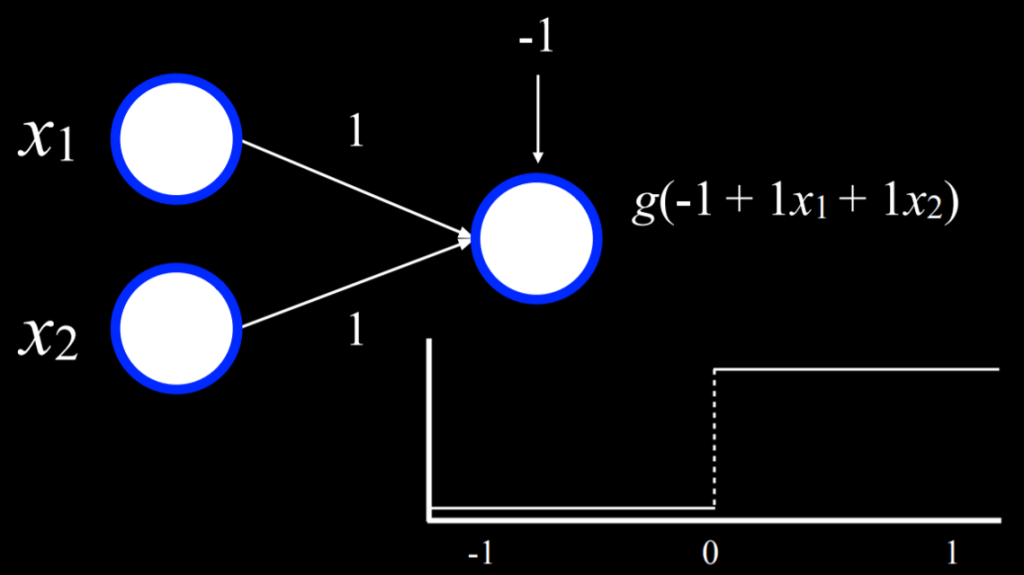
Here, the designated weights for each unit is equal to 1, and the function g outputs true if ≥ 0, and false if < 0. In case you haven’t noticed, this is the neural network equivalent of an “or” statement! Say that, for the inputs, false = 0 and true = 1. If x₁ = 0 and x₂ = 0, g(-1 + 1x₁ + 1x₂) = g(-1), outputting false, as -1 is below the threshold of 0. This intuitively makes sense: if x₁ is false and x₂ is false, the x₁ or x₂ should also be false. Now, imagine that either or both x₁ and x₂ = 1. g(-1 + 1x₁ + 1x₂) = g(0) or g(1), both of which output true, as both 0 and 1 meet the threshhold. Notice that we were able to express all of these scenarios in such a simple neural network operation.

Gradient Descent

Gradient descent serves as an algorithm to minimize loss during the training of neural networks. It essentially works as follows:

It first initiates with a random selection of weights: This step is simply a knowledgeless starting point in terms of appropriate weighting allocation for each input.

It then continuously iterates through the following steps:

1. Calculate the gradient by considering all data points that contribute to diminishing the loss
2. Adjust the weights in alignment with the calculated gradient

While this process is relatively simple and intuitive, it has a major drawback: to calculate gradients, it uses the entirety of data points, which leads to substantial computational costs. But many strategies exist to mitigate this issue. One approach is the Stochastic Gradient Descent, where gradient is calculated based on randomly chosen data points. Although this type of gradient might lose some accuracy, it is a relatively simple fix to the problem. It is important to note that there is no complete, flawless fix to this problem.

Leveraging gradient descent allows us to solve a multitude of challenges. Consider a scenario where the question is more nuanced than a simple “will it rain today?” By utilizing certain inputs, probabilities can be generated for diverse weather conditions. Subsequently, the most probable weather condition can be selected as the outcome. The diagram below shows the use of gradient descent when answering the question “what will be the weather like today?”:

This approach is applicable across various input-output configurations, where each input establishes connections with every output. These outputs correspond to actionable decisions. It’s essential to recognize that, in such neural networks, the outputs remain unconnected. Consequently, each output, along with its respective weights stemming from all inputs, can be regarded as an independent neural network. This independence permits separate training of each output in isolation from the others.

Because the concept of Neural Networks is difficult to grasp in the beginning, I will be continuing my discussion of this topic in my next blog post, this time talking about Multilayer Neural Networks, Backpropagation, etc. See you there!