The image above was created using AI. More specifically, this was the first image generated by Stable Diffusion, when given the prompt “AI Nim Harvard”.

Today officially marks the end of the fifth week of my participation in the Harvard Summer School Program. Since my last post on Minimax, there hasn’t been too much conceptual stuff I could talk about that really could fit on a blog format, as the Academic Integrity policy for CSCI S-80 does not allow for students to post their code solutions online, neither does it allow students to post pseudocode that can be translated into python code. However, this past week has taught me some of the ways AI models learn things.

Overall, there are three commonly used ways for AI to learn something. These categories are: supervised learning, unsupervised learning, and reinforcement learning. In this post, I will go through some of the more important concepts in Supervised Learning.

Supervised Learning

One task within supervised learning is Classification, where the computer maps an input to a discrete output. For example, it predicts whether it will rain on a given day based on humidity and air pressure, after being trained on a dataset with corresponding weather conditions.

The goal is to approximate a hidden function, f(humidity, pressure), that maps inputs to “Rain” or “No Rain.” By visualizing data points on a graph, we can see the challenge of predicting missing outputs (represented as white data points) solely based on input information. This can be seen in the following graphic:

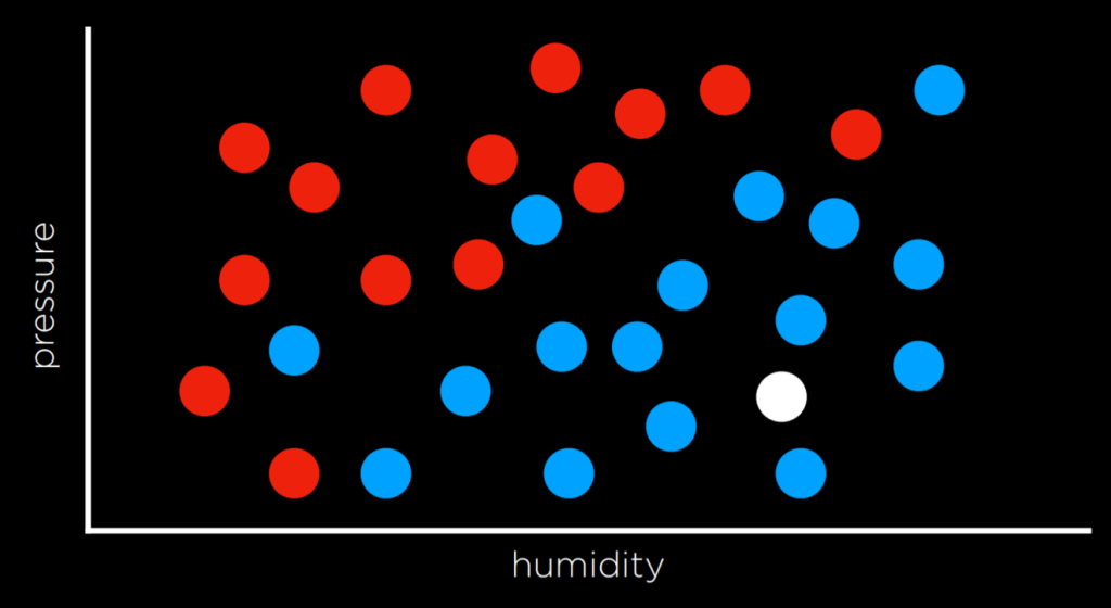
Solving tasks like this can be achieved by assigning the variable the value of its closest observation. For instance, in the graph, the white dot would be colored blue because the nearest observed dot is also blue. However, this simple approach might not always provide accurate results, as we can see in the following graphic:

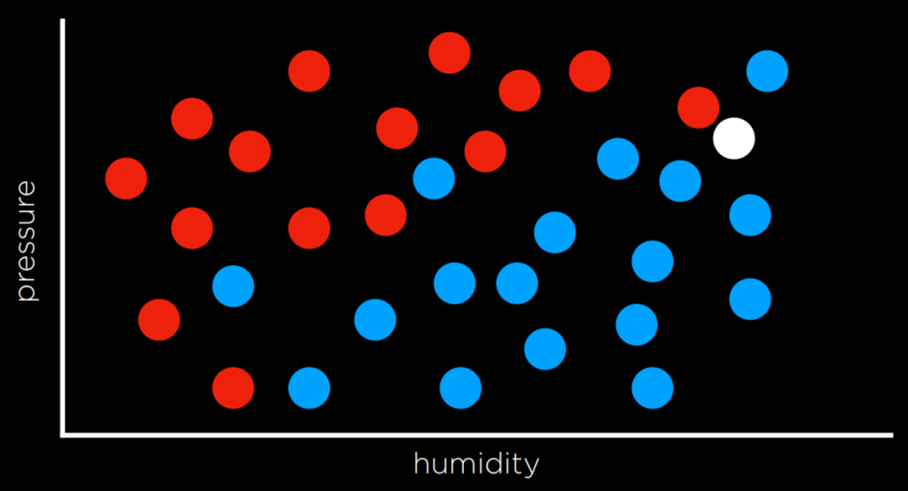
Here, because the dot closest to the white dot is red, nearest-neighbor classification might color it red. But looking at the dataset as a whole, it is pretty obvious that the dot should actually be colored blue.

To overcome the limitations of nearest-neighbor classification, an alternative is to use k-nearest-neighbors classification. In this method, the dot’s color is determined by the most frequent color among its k nearest neighbors. Choosing an appropriate value for k is essential. For example, with a 3-nearest neighbors classification, the white dot in the graph above would be colored blue, which appears to be a better decision. Nevertheless, k-nearest-neighbors classification is very expensive, as the algorithm needs to measure the distance of every single point to the point in question.

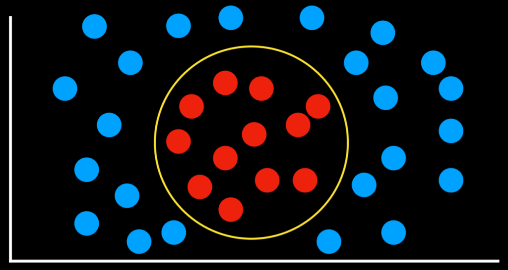
An alternative approach to tackle classification problems, instead of relying on nearest-neighbors, involves considering the data as a whole and establishing a decision boundary. We can see an example of this in the following chart:

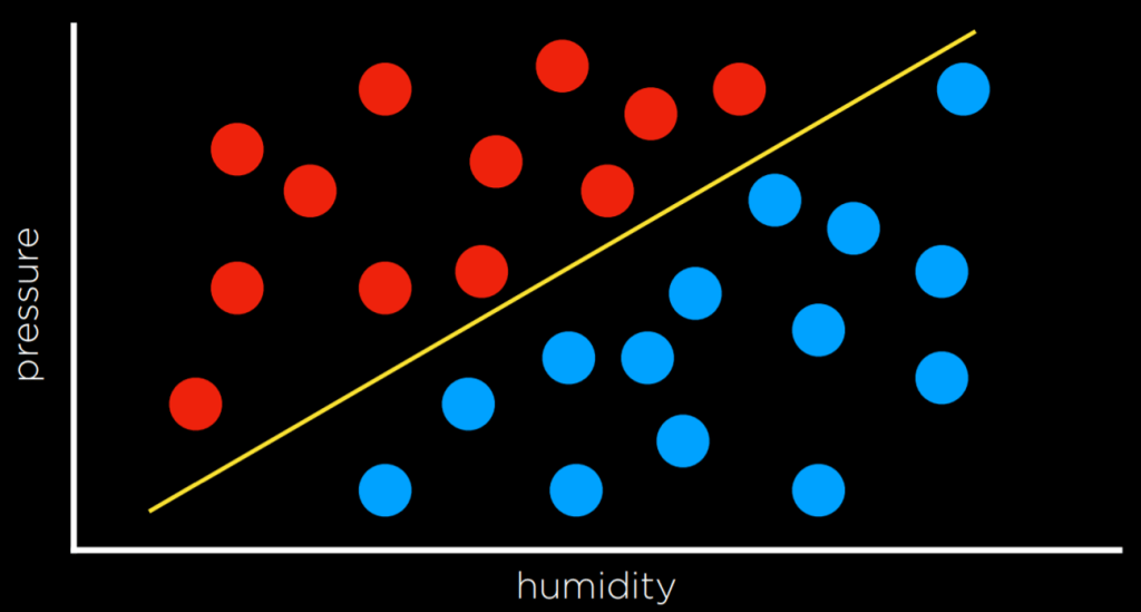
In two-dimensional data, this boundary can be a line that separates the two types of observations. Any additional data point will be classified based on which side of the line it falls on. However, this method has a drawback – real-world data tends to be very messy, making it challenging to draw a precise line that perfectly separates the classes without any errors. As a result, we often make compromises by drawing a boundary that mostly separates the observations correctly, but occasional misclassifications can still occur.

Apart from nearest-neighbor and linear regression, another classification approach is the Support Vector Machine. This method involves using an additional vector, called a support vector, near the decision boundary to make the most accurate decision when separating the data. While this increased accuracy might seem trivial, the following examples may help illustrate this point:

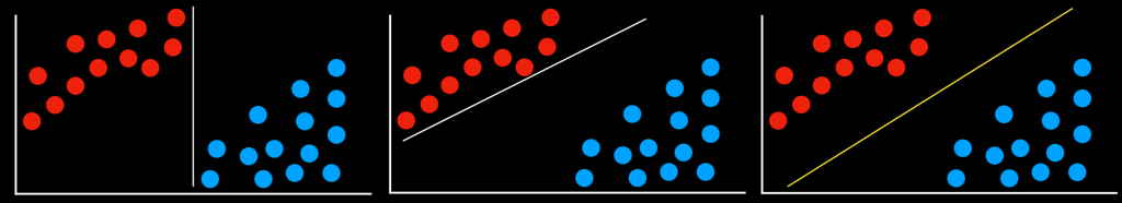
In all three of these scenarios, the decision boundary technically works: it doesn’t misclassify any points whatsover, dividing the red and blue dots correctly. However, it only takes a quick glance to tell that the third decision boundary is the best, as there is much more leeway for data variation without misclassification. Support Vector Machines maximize these margins, in addition to being able to generate decision boundaries that are not necessarily linear, like this one: